Graphs are my favorite abstract data type. I am not sure if my undergraduate education on graphs does the subject justice, but this is my attempt at summarizing the basic concepts and algorithms that I’ve learned in this area during university (minus spectral graph theory, I may dedicate a post to that later on). These algorithms are pretty timeless, so I’d like to have some personal documentation of them, intended to be read by someone who just wants a quick overview of the subject.
Table of Contents
- Defining Graphs
- Abstract Data Type Representations
- Breadth-First and Depth-First Search
- Shortest Paths
- Minimum Spanning Trees
- Directed Acyclic Graphs
- Network Flow
- Acknowledgements
Defining Graphs
In mathematics, graph theory is the study of graphs which are pairwise relations between objects.
An undirected graph is defined as the following ordered tuple \(G=(V, E)\) comprising of a set of vertices (aka nodes) \(V\) and a set of edges \(E \subseteq \{\{x,y\} ~ \\| ~ x,y \in V\}\), where these edges are unordered pairs of vertices. We can also have directed graphs, which are defined by the tuple \(G=(V, E)\), where \(E \subseteq \{\{x,y\} ~ \\| ~ x,y \in V^2\}\) is a set of ordered pairs of vertices rather than unordered. In a directed graph, an edge \(\{x, y\}\) is said to be directed from \(x\) to \(y\), meaning \(y\) is the successor of \(x\) and reachable from \(x\). In illustrations of directed graphs, there is an arrow at the head of the edge (successor) to show direction.
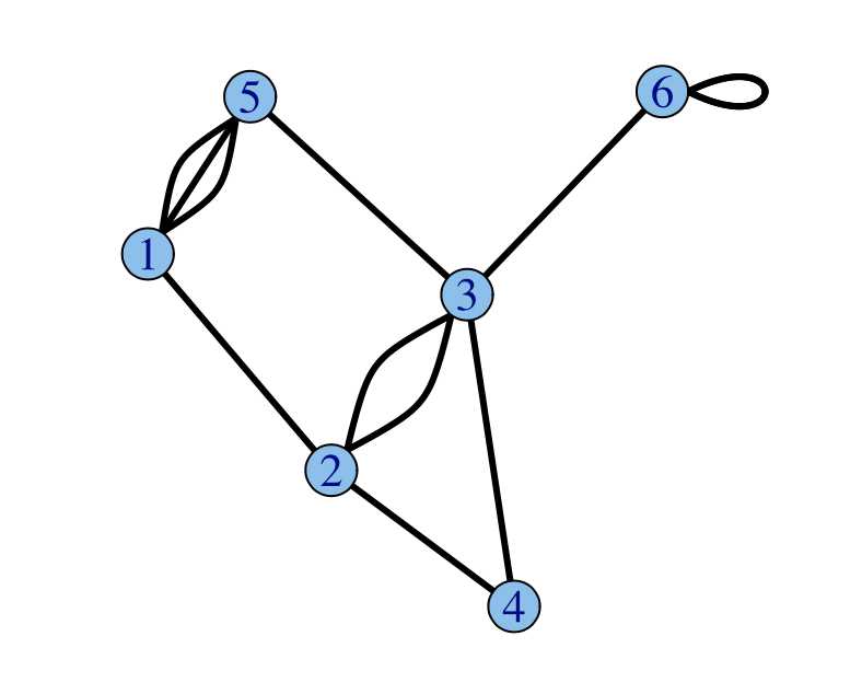
Graphs can contain loops (aka self-loops), which are edges that connect a vertex to itself. We can prohibit loops by modifiying the definition of our edges to be \(E \subseteq \{\{x,y\} ~ \\| ~ x,y \in V ~\text{and} ~x \neq y\}\) or \(E \subseteq \{\{x,y\} ~ \\| ~ x,y \in V^2 ~\text{and} ~x \neq y\}\) for directed graphs. Also we can permit multiple edges, which are two or more edges that are incident to the same two vertices (in directed graphs, these are edges such that they also hold the same direction too). To define this, we have the ordered triple \(G=(V,E,\phi)\), where \(E\) is the set of edges and \(\phi\) is a mapping for every edge to its unordered or ordered pair of vertices. We can define the following as \(\phi: E \rightarrow \{\{x,y\} ~ \\| ~ x,y \in V\}\) or \(\phi: E \rightarrow \{\{x,y\} ~ \\| ~ x,y \in V^2\}\) for directed graphs. We define a graph that allows multiple edges to be a multigraph. Otherwise, a graph without multiple edges is called a simple graph.
We define a connected component of an undirected graph as the induced subgraph in which any two vertices are connected to each other by paths, and which is connected to no additional vertices in the rest of the graph. We then define a graph to be connected if it has exactly one connected component, otherwise it is disconnected.
There are also a variety of special graphs, one such being a tree which is a connected acyclic graph. We define a cycle in an undirected graph as a non-empty trail (or directed trail for directed graphs) of vertices in which the only repeated vertices are the first and last vertices in the trail. Trees are usually seen in a hierarchial manner with a node being the root of the tree, in which all other nodes are illustrated going downwards.
Graphs can also have labels along their edges, such as words or numbers. We call graphs with numerical labels, weighted graphs.
With that said, there are many types of graphs that one can define which will not be covered here unless applicable (we define more graph types later).
Abstract Data Type Representations
Graphs are often used in computer science as an abstract data type. For example, they could represent a network of friends or a map of a city’s locations. In the one case, you might find it helpful to ask if a given two individuals are friends or not. In the other case, you might find that it is helpful to be able to construct a path from one location to another. Different graph implementations carry trade-offs with each other on how fast it takes to do these operations and how efficient it is to model these scenarios.
The first to examine is the adjacency list, a common implementation of graphs. It involves a collection of lists, where each list is the set of neighboring vertices for some vertex. One such implementation is a list of size \(n\) representing the \(n\) vertices numbered from \(0\) to \(n-1\). Each index \(i\) can hold a linked list of vertices that would be the vertices adjacent to vertex \(i\). There are other implementations that use hashtables to map vertices to their list of neighbors.
\(0: 1 \rightarrow 2 \rightarrow 3\)
\(1: 0 \rightarrow 3\)
\(2: 0\)
\(3: 4 \rightarrow 0 \rightarrow 1\)
\(4: 3\)
In this example of the adjacency list, we have an undirected graph with \(5\) vertices. Notice that since vertex \(3\) has \(0, 1,\) and \(4\) as its neighbors, those vertices also list \(3\) as their neighbor. In directed graphs, a vertex \(i\) lists a vertex \(j\) as its neighbor if and only if there is an edge directed from \(i\) to \(j\).
A benefit of an adjacency list is being able to represent sparse graphs (ones in which most pairs of vertices are not connected by edges) in a more space-efficient manner than the next implementation we will examine.
The main alternative to adjacency lists is the adjacency matrix. This is represented as an \(n\) by \(n\) matrix, such that the value at the index \((i, j)\) indicates whether vertices \(i\) and \(j\) share some edge. In directed graphs, this can be a one way relationship, such that \(A[i][j]\) indicates whether there is a directed edge from \(i\) to \(j\). In \(A[i][j]\), we can have some integer indicating the number of edges between \(i\) and \(j\), in which case \(0\) indicates no edge. There are different conventions for how to represent different relationships through the matrix. Based on the convention outlined, the following graph is undirected and we can also see that it is a symmetrical matrix, which is a property of undirected graphs.
\[\begin{bmatrix}1 & 0 & 1 & 0\\0 & 0 & 2 & 0\\ 1 & 2 & 0 & 1 \\ 0 & 0 & 1 & 0\\\end{bmatrix}\]A benefit of the adjacency matrix is the ability to determine if two vertices have an edge in \(\mathcal{O}(1)\) time. Also we can add or remove edges in \(\mathcal{O}(1)\), which the adjacency list doesn’t do as quickly in the worst case. However, the adjacency matrix is less space efficient, as it requires \(\mathcal{O}(\\|V\\|^2)\) space complexity, compared to its counterpart which requires less. If the graph is sparse, then the matrix will find itself filled with zeroes, a space inefficient representation of the absence of a relationship.
Breadth-First and Depth-First Search
The most important algorithms on graphs are searching algorithms. Being able to traverse the entire graph in a brute force manner allows us to accomplish many tasks.
    \begin{algorithm}
    \caption{Breadth First Search}
    \begin{algorithmic}
    \PROCEDURE{BFS}{$G, src$}
        \STATE $queue \leftarrow \emptyset$
        \STATE $visited \leftarrow \emptyset$
        \STATE $queue.$\CALL{add}{$src$}
        \STATE $visited.$\CALL{add}{$src$}
        \WHILE {$queue \neq \emptyset$}
            \STATE $u \leftarrow queue.$\CALL{remove}{}
            \FOR {$v \in G.adj[u]$}
                \IF {$v \notin visited$}
                    \STATE $visited.$\CALL{add}{$v$}
                    \STATE $queue.$\CALL{add}{$v$}
                \ENDIF
            \ENDFOR
        \ENDWHILE
    \ENDPROCEDURE
    \end{algorithmic}
    \end{algorithm}
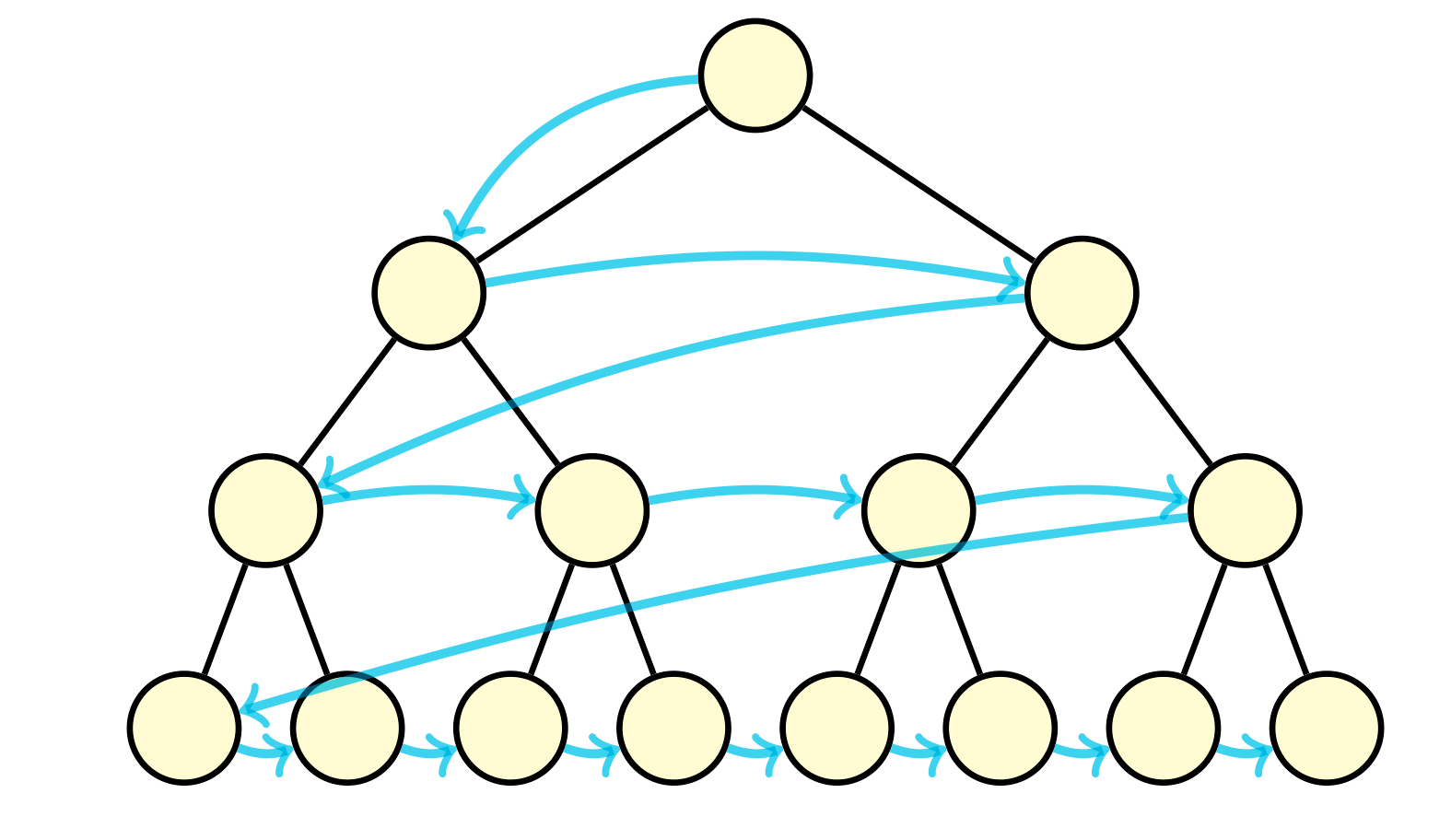
Breadth-first search is an algorithm that traverses the graph starting from a source vertex, level by level. We add the starting vertex to the queue, then as long as the queue is not empty, we remove a vertex from the queue, and append its undiscovered neighbors. This algorithm operates in time linear to the number of vertices and edges, \(\mathcal{O}(\\|V\\| + \\|E\\|)\).
There are an endless number of applications of BFS, here is a few. We can find a path between two vertices if we keep a track of the paths created by the traversal. This path that is found is actually the shortest path between two vertices on unweighted graphs. We can count the number of connected components by calling BFS on a set of unvisited vertices until we visited all the vertices in the set. We can determine if a graph is bipartite, which is a graph that can be partitioned into two sets of vertices \(U\) and \(V\) such that all edges connect a vertex in \(U\) to a vertex in \(V\). To determine if a graph is bipartite, we would need to ensure that we could color each vertex one of two colors such that no vertex has a neighbor with the same color. This can be done via BFS. Also to note, bipartite graphs do not contain odd-length cycles.
    \begin{algorithm}
    \caption{Depth First Search}
    \begin{algorithmic}
    \PROCEDURE{DFS}{$G, u, visited$}
        \STATE $visited.$\CALL{add}{$u$}
        \FOR {$v \in G.adj[u]$}
            \IF {$v \notin visited$}
                \STATE \CALL{DFS}{$G, v, visited$}
            \ENDIF
        \ENDFOR
    \ENDPROCEDURE
    \end{algorithmic}
    \end{algorithm}
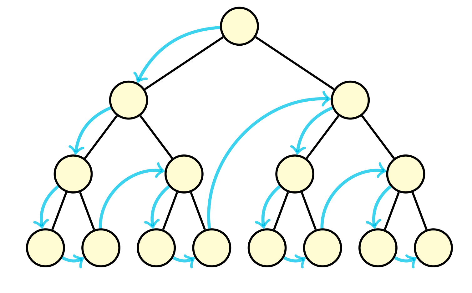
Depth-first search is the other fundamental algorithm for searching. It involves exploring as far as possible along some path before backtracking to explore other paths. This can be implemented using a stack, but is more often done recursively using the callstack. For each call of DFS, we examine a vertex’s neighbors, calling DFS again on one of its neighbors. Similar to BFS, we should mark vertices discovered as we visit them. And also similar to BFS, this algorithm operates in time linear to the number of vertices and edges, \(\mathcal{O}(\\|V\\| + \\|E\\|)\).
Similar to BFS, we can use DFS to find connected components and even determine if a graph is bipartite. However, there are various applications of DFS that BFS cannot solve. For example, DFS allows us to find cycles in directed graphs, which does not work in BFS.
In general, these two algorithms are very powerful. Many problems involving graphs are solved using modifications of BFS and DFS.
Shortest Paths
While BFS is useful for finding shortest paths in unweighted graphs, it fails to capture the shortest paths in weighted graphs, where each edge contains a numerical label that indicates the cost of traversing that edge.
    \begin{algorithm}
    \caption{Dijkstra's}
    \begin{algorithmic}
    \PROCEDURE{Dijkstras}{$G, src$}
        \STATE $queue \leftarrow \emptyset$
        \STATE $dist \leftarrow \emptyset$
        \STATE $parent \leftarrow \emptyset$
        \FOR {$v \in G$}
            \IF {$v \neq src$}
                \STATE $dist[v] \leftarrow \infty$
                \STATE $parent[v] \leftarrow null$
                \STATE $queue.$\CALL{enqueue-priority}{$v, dist[v]$}
            \ENDIF
        \ENDFOR
        \STATE $dist[src] \leftarrow 0$
        \STATE $queue.$\CALL{enqueue-priority}{$src, dist[src]$}
        \WHILE {$queue \neq \emptyset$}
            \STATE $u \leftarrow queue.$\CALL{extract-min}{}
            \FOR {$v \in G.adj[u]$}
                \STATE $alt = dist[u] + $\CALL{cost}{$u, v$}
                \IF {$alt < dist[v]$}
                    \STATE $dist[v] \leftarrow alt$
                    \STATE $parent[v] = u$
                    \STATE $queue.$\CALL{decrease-priority}{$v, alt$}
                \ENDIF
            \ENDFOR
        \ENDWHILE
        \RETURN{$dist, parent$}
    \ENDPROCEDURE
    \end{algorithmic}
    \end{algorithm}
Dijkstra’s algorithm is one of the most famous graph traversal algorithms. It only works on weighted graphs in which the weights are positive values. It finds the shortest path to all vertices from some source vertex \(src\). The proof of this algorithm is by induction. Without going into the weeds with this induction, the intuition for it is that of a greedy approach. The idea that if there was a better path than the one we just evaluated, we would have visited that path before hand. This algorithm can take \(\mathcal{O}((\\|V\\| + \\|E\\|)log(\\|V\\|))\) if we use a binary heap for our priority queue. Using a fibonacci heap we can improve to \(\mathcal{O}(\\|E\\| + \\|V\\|log(\\|V\\|))\).
    \begin{algorithm}
    \caption{A* Search}
    \begin{algorithmic}
    \PROCEDURE{Astar}{$G, src, dst$}
        \STATE $queue \leftarrow \emptyset$
        \STATE $set \leftarrow \emptyset$
        \STATE $dist \leftarrow \emptyset$
        \STATE $parent \leftarrow \emptyset$
        \FOR {$v \in G$}
            \IF {$v \neq src$}
                \STATE $dist[v] \leftarrow \infty$
                \STATE $parent[v] \leftarrow null$
            \ENDIF
        \ENDFOR
        \STATE $dist[src] \leftarrow 0$
        \STATE $queue.$\CALL{enqueue-priority}{$src, dist[src]$}
        \WHILE {$queue \neq \emptyset$}
            \STATE $u \leftarrow queue.$\CALL{extract-min}{}
            \IF {$u == dst$}
                \RETURN {$u, dist, parent$}
            \ENDIF
            \STATE $set.$\CALL{add}{u}
            \FOR {$v \in G.adj[u]$}
                \IF {$v \notin set$}
                    \STATE $alt \leftarrow dist[u] +$ \CALL{cost}{$u, v$}
                    \IF {$alt < dist[v]$}
                        \STATE $dist[v] \leftarrow alt$
                        \STATE $parent[v] = u$
                        \STATE $queue.$\CALL{enqueue-priority}{$v, alt + $\CALL{heuristic}{$v$}}
                    \ENDIF
                \ENDIF
            \ENDFOR
        \ENDWHILE
        \RETURN{$failure$}
    \ENDPROCEDURE
    \end{algorithmic}
    \end{algorithm}
A* search is an efficient algorithm for finding the shortest path between two vertices in a weighted graph. We can view it as an extension of Dijkstra’s algorithm with this added heuristic that guides our search. For example, this heuristic can be the Euclidean distance between destination and the given vertex. At each iteration, it decides which vertex \(u\) to visit next based on this value \(\text{f}(u) = \text{dist}[u] + \text{heuristic}(u)\). This algorithm has a similar time complexity to Dijkstra’s algorithm, although it is likely to terminate earlier due to pruning paths along its search.
    \begin{algorithm}
    \caption{Bellman-Ford}
    \begin{algorithmic}
    \PROCEDURE{BellmanFord}{$G, src$}
        \STATE $dist \leftarrow \emptyset$
        \STATE $parent \leftarrow \emptyset$
        \FOR {$v \in G$}
            \IF {$v \neq src$}
                \STATE $dist[v] \leftarrow \infty$
                \STATE $parent[v] \leftarrow null$
            \ENDIF
        \ENDFOR
        \STATE $dist[src] \leftarrow 0$
        \STATE $N \leftarrow G.$\CALL{num-vertices}{}
        \FOR {$i=1$ \TO $N-1$}
            \FOR {$\{u, v\} \in G.$\CALL{edges}{}}
                \IF {$dist[u] + $\CALL{cost}{$\{u, v\}$} $< dist[v]$}
                    \STATE $dist[v] \leftarrow dist[u] + $\CALL{cost}{$\{u, v\}$}
                    \STATE $parent[v] \leftarrow u$
                \ENDIF
            \ENDFOR
        \ENDFOR
        \FOR {$\{u, v\} \in G.$\CALL{edges}{}}
            \IF {$dist[u] + $\CALL{cost}{$\{u, v\}$} $< dist[v]$}
                \RETURN{failure}
            \ENDIF
        \ENDFOR
        \RETURN{$dist, parent$}
    \ENDPROCEDURE
    \end{algorithmic}
    \end{algorithm}
The Bellman-Ford algorithm accomplishes the task of finding a shortest path from a single vertex to all vertices in a weighted directed graph. The advantage to this algorithm over Dijkstra’s algorithm is that it works on weighted graphs with negative weights. The issue found within Dijkstra’s algorithm occured when we had a negative cycle, defined as a cycle in which the sum of the weights are negative. To gain a more negative cost path in this case, Dijkstra’s would iterate through the cycle an infinite number of times. To combat this, Bellman-Ford is able to detect if a negative cycle exists. The essence is in the fact that the maximum length of a path is \(\\|V\\| - 1\), in which we improve our paths by 1 edge each iteration by brute forcing over all edges. This is why when we do a final pass after \(\\|V\\| - 1\) iterations, a decrease in the cost of any path indicates a negative cycle. Bellman-Ford is slower than Dijkstra’s algorithm, performing in \(\mathcal{O}(\\|V\\|\\|E\\|)\).
Minimum Spanning Trees
A minimum spanning tree of a connected weighted graph \(G = (V, E)\) is a connected graph \(G' = (E', V')\) such that \(E' \subseteq E\), \(\\|E'\\| = \\|V\\| - 1\), and \(\sum_{\{u, v\} \in E'} cost(\{u, v\})\) is minimal. In other words, a minimum spanning tree of \(G\) is a tree that includes all vertices of \(G\) and whose total edge weight cost is minimal. There are two popular algorithms for finding these minimum spanning trees.
    \begin{algorithm}
    \caption{Prim's}
    \begin{algorithmic}
    \PROCEDURE{Prims}{$G$}
        \STATE $visited \leftarrow \emptyset$
        \STATE $MST \leftarrow \emptyset$
        \STATE $x \leftarrow \text{arbitrary vertex} \in G$
        \STATE $visited.$\CALL{add}{$x$}
        \WHILE {$visited.$\CALL{size}{} $\neq G.$\CALL{num-vertices}{}}
            \STATE $\{u, v\} \leftarrow \text{lowest cost edge such that } u \in visited \text{ and } v \notin visited$
            \STATE $MST.$\CALL{add}{$\{u,v\}$}
            \STATE $visited.$\CALL{add}{$v$}
        \ENDWHILE
        \RETURN{$MST$}
    \ENDPROCEDURE
    \end{algorithmic}
    \end{algorithm}
Prim’s algorithm finds the MST by greedily building the tree by examining the next lowest cost edge that we can add to the tree without creating a cycle in the tree. Each step connecting the tree to a vertex not in the tree yet. This algorithm can run in \(\mathcal{O}(|E|log(|V|))\) using a priority queue. We would use Prim’s when the graph is dense (number of edges is high).
    \begin{algorithm}
    \caption{Kruskal's}
    \begin{algorithmic}
    \PROCEDURE{Kruskals}{$G$}
        \STATE $U \leftarrow \text{disjoint-set data structure}$
        \STATE $MST \leftarrow \emptyset$
        \FOR {$v \in G$}
            \STATE $U.$\CALL{make-set}{$v$}
        \ENDFOR
        \FOR {$\{u,v\} \in G.$\CALL{edges}{} $\text{ordered by nondecreasing weight}$}
            \IF {$U.$\CALL{find-set}{$u$} $\neq U.$\CALL{find-set}{$v$}}
                \STATE $MST.$\CALL{add}{$\{u,v\}$}
                \STATE $U.$\CALL{union}{$u, v$}
            \ENDIF
        \ENDFOR
        \RETURN{$MST$}
    \ENDPROCEDURE
    \end{algorithmic}
    \end{algorithm}
Kruskal’s algorithm builds the MST using a disjoint-set (union-find) data structure. Initially all the vertices are in their own sets. We build our tree by greedily combining these sets by looking at the lowest cost edge. This algorithm runs in \(\mathcal{O}(\\|E\\|log(\\|E\\|))\).
Directed Acyclic Graphs
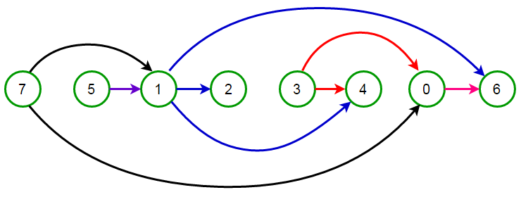
Directed acyclic graphs appear in many places and luckily they have a neat property. We can obtain a topological ordering on the vertices, giving us an ordering in which all edges are directed from left to right. When operating on directed acyclic graphs in algorithm design, it is almost always a wise decision to apply a topological sort first. It is also very important to note that all directed acyclic graphs have a topological ordering and all graphs with a topological ordering are directed acyclic graphs.
    \begin{algorithm}
    \caption{Topological Sort}
    \begin{algorithmic}
    \PROCEDURE{TopologicalSort}{$G$}
        \STATE $L \leftarrow \emptyset$
        \WHILE {$\exist v \in G \text{ that is not permanently marked}$}
            \STATE \CALL{DFS}{$G, v, L$}
        \ENDWHILE
        \RETURN{$L$}
    \ENDPROCEDURE
    \PROCEDURE{DFS}{$G, v, L$}
        \IF {$v \text{ is permanently marked}$}
            \RETURN{}
        \ENDIF
        \IF {$v \text{ is temp marked}$}
            \STATE \textbf{stop}
        \ENDIF
        \STATE $\text{temp mark }v$
        \FOR {$u \in G.adj[v]$}
            \STATE \CALL{DFS}{$G, u, L$}
        \ENDFOR
        \STATE $\text{remove temp mark }v$
        \STATE $\text{permanently mark }v$
        \STATE $L.$\CALL{append}{$v$}
    \ENDPROCEDURE
    \end{algorithmic}
    \end{algorithm}
This algorithm deploys a depth first search and therefore it performs in \(\mathcal{O}(\\|E\\| + \\|V\\|)\). The idea is in constructing the order backwards, in which we stop calling the visit DFS once we hit a marked vertex or a vertex with outdegree equal to \(0\).
    \begin{algorithm}
    \caption{Kahn's}
    \begin{algorithmic}
    \PROCEDURE{Kahns}{$G$}
        \STATE $L \leftarrow \emptyset$
        \STATE $S \leftarrow \emptyset$
        \FOR {$v \in G$}
            \IF {$v \text{ has no incoming edge}$}
                \STATE $S.$\CALL{add}{$v$}
            \ENDIF
        \ENDFOR
        \WHILE {$S \neq \emptyset$}
            \STATE $v \leftarrow S.$\CALL{remove}{}
            \STATE $L.$\CALL{append}{$v$}
            \FOR {$u \in G.adj[v]$}
                \STATE $G.$\CALL{remove}{$\{v,u\}$}
                \IF {$u \text{ has no incoming edges}$}
                    \STATE $S.$\CALL{add}{$u$}
                \ENDIF
            \ENDFOR
        \ENDWHILE
        \RETURN{$L$}
    \ENDPROCEDURE
    \end{algorithmic}
    \end{algorithm}
Another algorithm for determining a topological ordering is Kahn’s algorithm. This also performs in \(\mathcal{O}(\\|E\\| + \\|V\\|)\). The order in which the ordering is built is also the order of the ordering. Each time we add a vertex \(v\) to the ordering, that vertex has \(0\) incoming edges. Upon adding the vertex to the ordering, we also examine the vertices adjacent to it, denoted \(u\), in which we remove this edge \(\{v, u\}\) from the graph. Then adding to our set of vertices with \(0\) incoming edges, any new vertices with \(0\) incoming edges now.
Network Flow
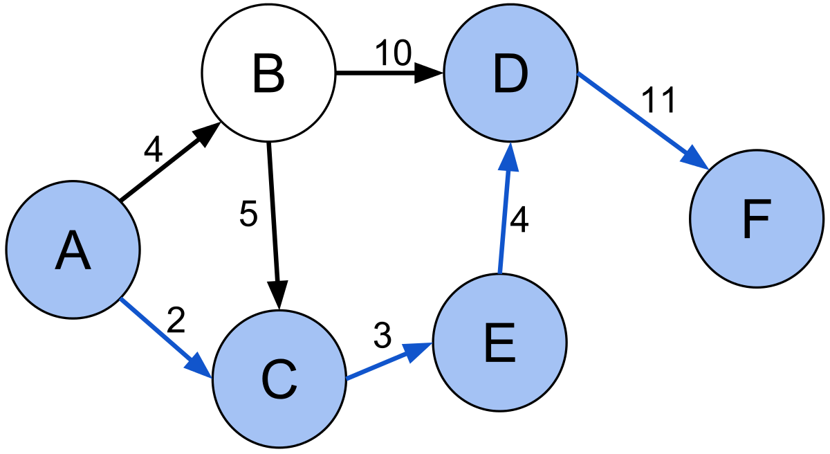
In flow network models, we have a directed graph \(G\) with capacities along its edges. Suppose we want to send flow along the edges, knowing that these flow amounts cannot exceed the capacities of the edges. We will have a source vertex \(s\) that emits the flow and a sink vertex \(t\) that collects the flow. We want to compute the maximum amount of flow that we can send in our network.
An \(s-t\) cut of a flow network \((G = (V, E), s, t, c)\) where \(c\) is the cost of the edges, is a partition of \(V\) into two sets \(S\) and \(T\) where \(s \in S\) and \(t \in T\). The capacity of a cut \(C(S, T)\), denoted \(c(S, T)\), is the sum of the capacities of the edges \((u, v)\) with \(u \in S\) and \(v \in T\). That being: \(c(S, T) = \sum_{\{u,v\} : u \in S, v \in T} c(\{u,v\})\).
The flow of a cut \(C(S, T)\) is the amount of flow that crosses from \(S\) to \(T\), denoted \(f(S, T)\) and is defined as \(f(S, T) = (\sum_{\{u, v\}:u \in S, v \in T} f(u ,v) - \sum_{\{v, u\}: v \in T, u \in S} f(v, u))\). The flow across a cut is equal to the flow that leaves \(s\).
A useful theorem to note is the max-flow min-cut theorem. It asserts that the maximum amount of flow \(f\) that can pass from the source \(s\) to the sink \(t\) is equal to the capacity of the minimum \(s-t\) cut.
    \begin{algorithm}
    \caption{Ford-Fulkerson}
    \begin{algorithmic}
    \PROCEDURE{FordFulkerson}{$G$}
        \STATE $f \leftarrow 0$
        \FOR {$\{u,v\} \in G.$\CALL{edges}{}}
            \STATE \CALL{flow}{$u, v$} $\leftarrow 0$
        \ENDFOR
        \WHILE {$\exist \text{ path } p \text{ from } s \text{ to } t \text{ in } G_f \text{ s.t. } c_f > 0 \text{ for all edges } \{u,v\} \in p$}
            \STATE $bottleneck \leftarrow min\{$\CALL{cost}{$u, v$}$: \{u, v\} \in p\}$
            \STATE $f \leftarrow f + bottleneck$
            \FOR {$\{u, v\} \in p$}
                \IF {$\{u, v\} \in G.$\CALL{edges}{}}
                    \STATE \CALL{flow}{$u, v$} $\leftarrow$ \CALL{flow}{$u, v$} $ + bottleneck$
                \ELSE
                    \STATE \CALL{flow}{$v, u$} $\leftarrow$ \CALL{flow}{$v, u$} $ - bottleneck$
                \ENDIF
            \ENDFOR
        \ENDWHILE
        \RETURN{$f$}
    \ENDPROCEDURE
    \end{algorithmic}
    \end{algorithm}
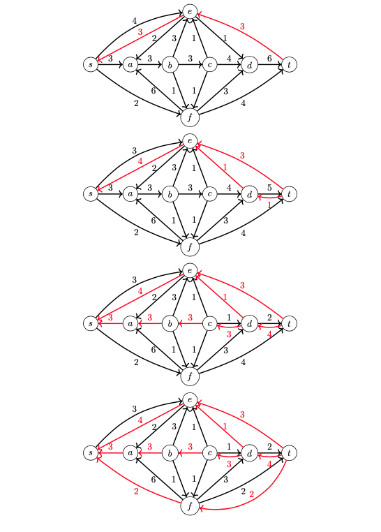
There is a useful algorithm for computing the maximum flow of a flow network and it is called the Ford-Fulkerson algorithm. Each iteration of the algorithm, we find an existing path in our flow network, pushing the maximum flow we can along that path. The pushing of the flow will give us edges in the opposite direction of each edge on the path, with the capacity of the flow. As such, we consider edges that are in the original graph forward edges and the edges that go in the opposite direction as backward edges. Once we exhaust all the paths that we can push flow along, whatever vertices are reachable by \(s\) still, creates the \(S\) partition in the cut.
Acknowledgements
I acknowledge the following courses at the Univeristy of Washington for teaching me much of what I know about graph theory: CSE 311 (Foundations), CSE 331 (SWE), CSE 332 (Data Structures), CSE 417 (Algos + Complexity), CSE 446 (ML), CSE 421 (Algos), and CSE 490Z1/422 (Modern Algos). I also acknowledge the Google search engine and its web results for helping me formalize my previous knowledge as well as teaching me things that I never knew I wanted to know (never occurred to me that I could do a topological sort with simple DFS calls).